Spreadsheet Activity #8:   Linear Regression - Standard Curve of Absorbance Data for Dye Analysis

[Back to Group 1 Assignments] [Back to Chem3020 home]

One of the most basic plotting techniques is to create a standard [calibration] curve. Chemical solutions of known concentrations are measured on an instrument and then the resulting signals are plotted as a function of concentration to obtain a "standard curve." With a slope and intercept, a linear function can then be solved to obtain concentrations from instrumental signals when determining unknown solutions.

Linear fit for data points:          y = m * x + b
Determination of Unknowns:   x = (y - b) / m

(Where m=slope and b=intercept)

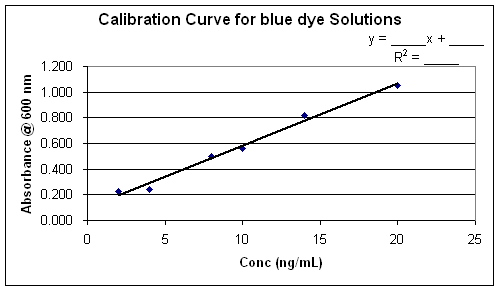
Plot the following data for the calibration of blue dye in aqueous solution. Be sure to plot the concentrations on the x-axis and the absorbance values on the y-axis.

Add a trend line to your data points. In Excel, right click on the data series on the chart and select “Add Trendline.” From the menu box, select a linear fit and then click on the “options” tab and check the options to display both the equation and R-squared. Type these values that are displayed on your chart into the spreadsheet where indicated (below “Values from Trend Line.”

Also calculate the slope, intercept and R-squared in separate cells on your spreadsheet in the appropriate cells beneath “Your Calculations.”

Using the formula above (x=(y-b)/m) and your calculated slope and intercept values, calculate the concentration of the three unknown solutions with absorbance values of: 0.623, 0.304, 2.312.

(Click here to download data: 8BlueDye)

Experimental Data from Analysis of Blue Dye Solution:

Conc.	Abs.	.	Your Calculations (Cell Formulas):
(ng/mL)	(600nm)	Slope:	.
2	0.228	Intercept	.
4	0.245	R^2	.
8	0.499	.	Values From Trend Line (on Chart):
10	0.561	Slope:	.
14	0.819	Intercept	.
20	1.055	R^2:	.
Unknowns	Abs.
	0.623
	0.304
	2.312

Question: Do you think that this calibration is appropriate for the last unknown in the list (Abs = 2.312)?

Comment on this in your report.

Example Chart:

Excel Programming Tips:

Excel command:	Result
=SLOPE(Y range, X range)	Calculates the Slope of the values given.
=INTERCEPT(Y range, X range)	Calculates the Intercept of the values given.
=RSQ(Y range, X range)	Calculates the R^2 of the values given.

Note: If you used the Calculated values for Slope and intercept in your unknown determination, you can make changes to your data points and see the effect on the unknowns’ concentrations. This is particularly useful when you need to change something (such as a typo) in a large spreadsheet with many calculations.